Integrate Classiq into your app
Quickly turn any optmization problem into a quantum computing program using Classiq. Here I show how to optimize a portfolio of stocks using Classiq, and exposing that via a web app.


Quantum computing is now still in the academic phase. This can also be seen in the tools that are commonly used, like Qiskit, Q#, and Cirq. These are all very powerful but not easy to learn for everyone. One of the goals of Classiq is to make quantum computing more accessible. Here I will show how I integrated a common QAOA algorithm into a web app, making it accessible even for people without any understanding of quantum computing.
Problem statement
The application we want to create is a portfolio optimization solver. Given some stocks and optimization parameters, we want a quantum computer or simulator to give the optimal distribution of assets.
Writing the quantum code
This might sound like the hard part, but lucky for us, that is not the case when using Classiq. You do not need any quantum knowledge to create a QAOA optimization quantum circuit. The only requirement is to be able to describe your problem in the Pyomo package. Let's first think of what the code would need to do.
- Be able to set a budget and not exceed this. Unfortunately, we do not have unlimited money.
- Set a specific max budget per asset. We might not want to put all our eggs in one basket.
- Optimize the total return compared to some risks we are willing to take.
- be able to trade off more risk to get higher returns.
We will first start with the description of the assets that we could pick from. In this example, we have three possible assets two have positive historical returns and one a negative return. Next to returns, we also have the covariance between the assets. This describes the relation between the assets. For example, when one asset would go up, would the other also move up or move down. Lastly, we have the total budget that we can spend, in this case, that is the number of assets that we can buy. so the price of assets is not taken into account here, and there is a maximum number of positions per asset. All this is represented like this:
returns = np.array([3, 4, -1])
# fmt: off
covariances = np.array(
    [
        [ 0.9,  0.5, -0.7],
        [ 0.5,  0.9, -0.2],
        [-0.7, -0.2,  0.9],
    ]
)
# fmt: on
total_budget = 6
specific_budgets = [2, 2, 2]
Now let's write the optimization code in Pyomo.
portfolio_model = pyo.ConcreteModel("portfolio_optimization")
num_assets = len(returns)

# setting the variables
portfolio_model.w = pyo.Var(
    range(num_assets),
    domain=pyo.Integers,
    bounds=lambda _, idx: (0, specific_budgets[idx]),
)
w_array = list(portfolio_model.w.values())

# setting the constraint
portfolio_model.budget_rule = pyo.Constraint(expr=(sum(w_array) == total_budget))

# setting the expected return and risk
portfolio_model.expected_return = returns @ w_array
portfolio_model.risk = w_array @ covariances @ w_array

# setting the cost function to minimize
portfolio_model.cost = pyo.Objective(
	expr=portfolio_model.risk - lamda_value * portfolio_model.expected_return, sense=pyo.minimize
)
Let's walk quickly through what is done without diving too deep into it.
- We create a Pyomo model
ConcreteModel("")this will describe the optimization problem. - Next, we declare the variables, there is one variable per asset, and each variable is an integer, representing the number of positions in a specific asset. With the bounds function, we make sure the specific budget for each asset is not exceeded
- the
w_arraywill hold the total number of positions per asset - In the budget rule, we make sure the total budget is not exceeded
- Next, given the covariance and historical returns, we calculate the risk and expected return.
- Finally, we have an objective function that minimizes the risk while optimizing the return.
That is all no quantum computing knowledge is required, and this model could be solved with a classical solver. However, the goal is to solve this with a quantum computer. Enter Classiq.
We can create a quantum program from this classical optimization problem with just a few extra lines of code. First, we set the quantum properties of the problem, namely the number of layers in the QAOA problem. Like with neural networks, in QAOA, you can add one or more layers to solve the problem. This is done with a simple line of code. Later you will see this can be adjusted easily.
qaoa_config = QAOAConfig(num_layers=1)QAOA is a hybrid algorithm, meaning that part of the calculation still is done classically. In the quantum program, some parameters could be tweaked. The goal of the classical optimizer is to find the optimal values for these parameters. It is possible to manage how the classical optimizer works. For example, set the number of times the QAOA circuit should be executed and what results should be used for the optimization. In this case, we optimize 70% of the best results of the previous run. Setting this and more can be done in a single line.
optimizer_config = OptimizerConfig(max_iteration=60, alpha_cvar=0.7)Finally, we will combine everything in the Classiq model and execute the circuits.
model = construct_combinatorial_optimization_model(
pyo_model=portfolio_model,
qaoa_config=qaoa_config,
optimizer_config=optimizer_config,
)
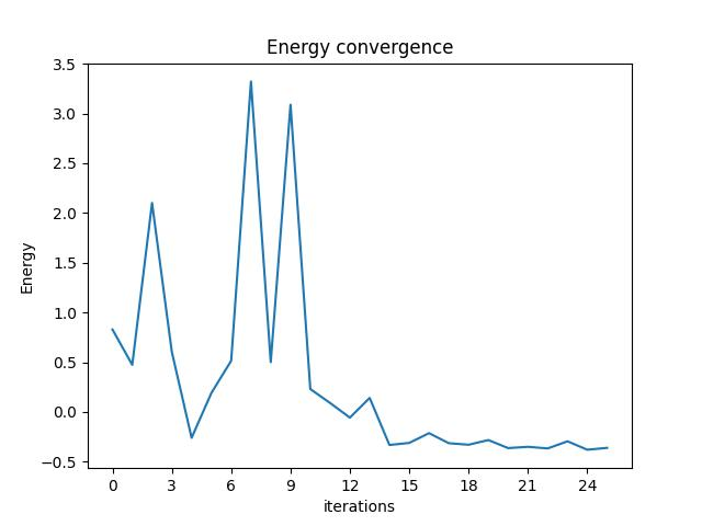
res = execute(qprog)The result contains both the optimized portfolio and the energy convergence graph:
| probability | cost | solution | count |
|---|---|---|---|
| 0.005859 | -4.8 | [1, 2, 1] | 12 |
| 0.003906 | -4.8 | [1, 2, 1] | 8 |
| 0.003906 | -4.8 | [2, 1, 1] | 8 |
| 0.004395 | -4.8 | [2, 1, 1] | 9 |
| 0.003906 | -4.8 | [2, 1, 1] | 8 |
As you can see, the best portfolio buys one share of asset 1, two of asset 2, and one of asset 3.
Let's integrate this into a web app
The goal here was to make this as accessible as possible, and even though I think the code optimization code can not be simplified any further, not everyone runs Python on their machine. So to make it as accessible as possible, I created a web app which is shown below. This was quite easy because Classiq has an easy Python SDK, which can easily be integrated into a FastAPI. I created 3 endpoints, but you could also use a single endpoint. This was my result:
#create the model which we described above
@router.post("/portfolio")
def calculate_port_model(portfolio: PortfolioModel):

    # Inser the pyomo code here

    return pyomo model

#Synthesise the created model
@router.post("/synthesize")
async def synthesize_model(model: SynthesizeModel):
	qprog = await synthesize_async(json.dumps(model))
    return qprog

#Finaly execute the circuit
@router.post("/execute")
async def execute_qprog(qprog: ExecuteModel):
    result = await execute_async(json.dumps(qprog))
    return result
As you can see in the first endpoint, I created the Pyomo model. This is passed to the front end, so the user can see this intermediary result.
The next endpoint will take the Pyomo model that was created and synthesize that using the Classiq synthesis engine into a real quantum program that can run on a quantum computer.
Finally, the quantum code is executed in the last call.
Which leaves only to create a web front end. The code can be found on this Github. The whole process works as follows:
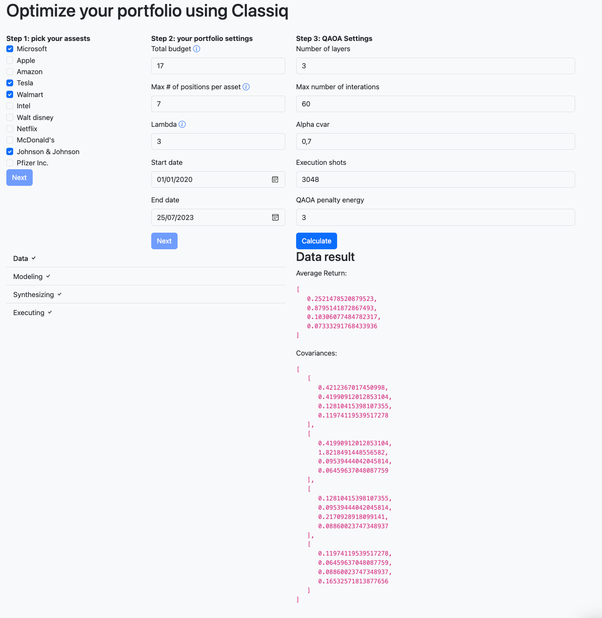
- Select the stocks you want to consider for the optimization. The stock data will be loaded from Yahoo Finance to ensure up-to-date data is always used.
- Next, you can set some details about the portfolio that you want to create. In this case, we assume that all assets are priced the same.
You can set a max number of positions per asset.
The lambda is a trade-off between risk and reward. The higher the number, the higher the risk. Lastly, the date selector allows the users to select a time frame to fetch the returns and covariance data.
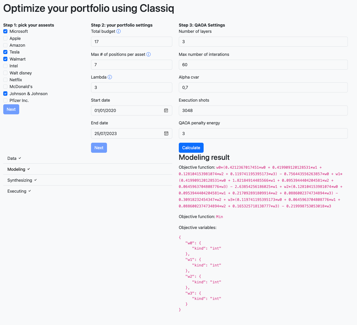
Below you see the result of these two first phases. On the left, you see the raw data, the returns, and covariances. On the right, you see the result of the Pyomo, the expression which should be optimized.
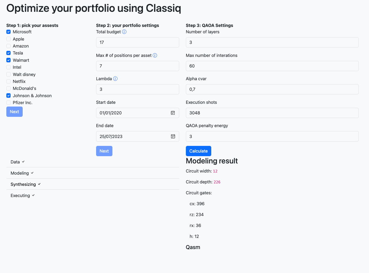
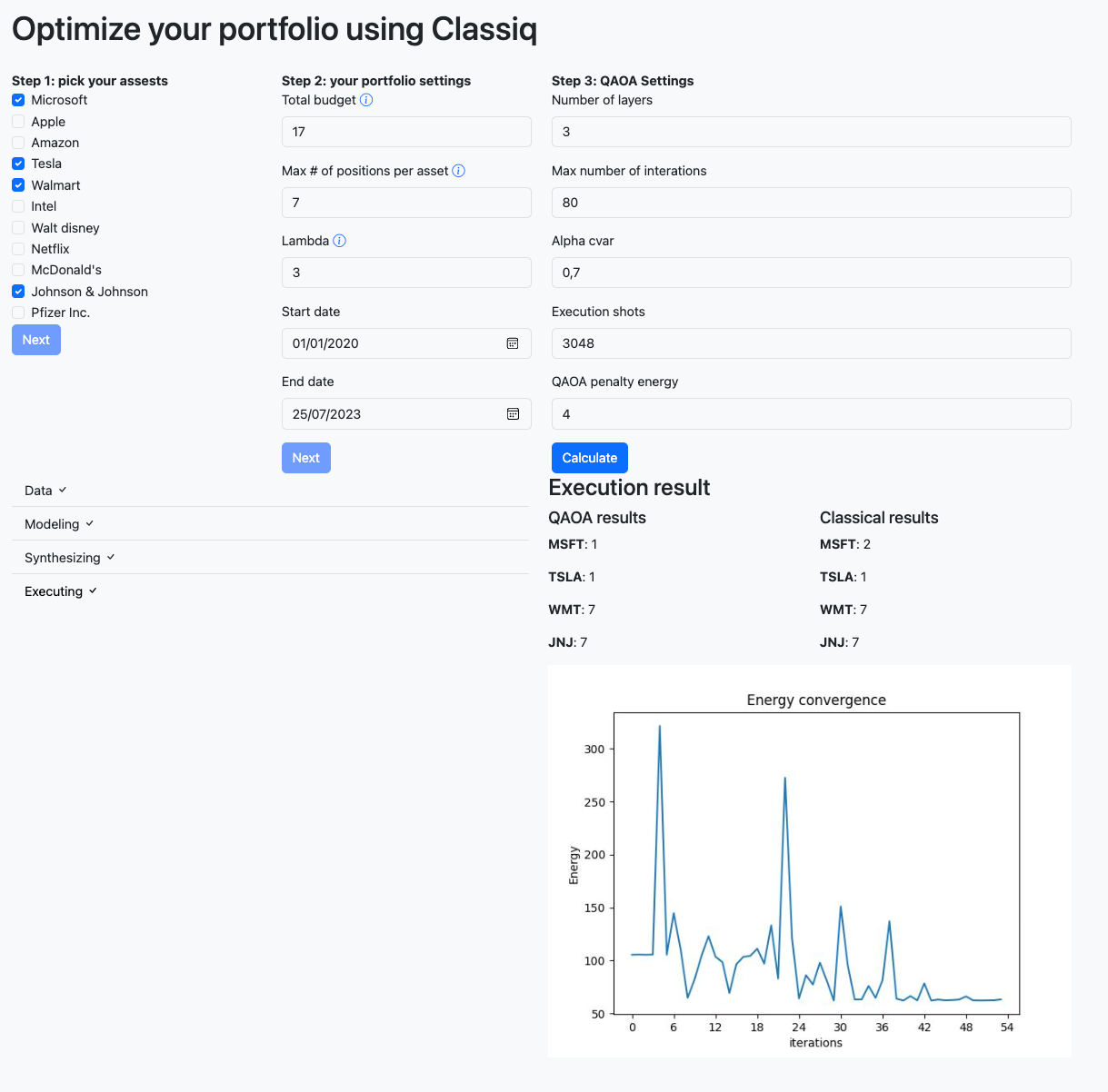
- In the QAOA settings part, setting some parameters that we have seen before is possible. This will generate a quantum circuit, which results you can see below. You will see the depth and width of the circuits as well as the gates that are used.
Finally, let's look at the results. You can see how the energy graph converges to the lowest energy level, as you can see, the lowest level is reached before the maximum number of iterations. As you can see, both the classical and quantum optimization results are almost the same, which means the global minima are probably found.
Conclusion
I hope this shows how easy it is to formulate optimization problems using Classiq and turn them into real quantum programs without any quantum knowledge. This is just a single example. With this base, it is really easy to integrate more Classiq solutions into day-to-day applications.