Quantum inspired optimization - Traveling salesperson
How to use Quantum Inspired Compute to calculate the shortest possible route for the traveling salesperson problem. Here we are using Azure quantum to solve the TSP problem. We firstly create the QUBO from Bing maps data, and then solve this using Azure Quantum.


In February 2021 Microsoft announced this awesome new Azure service Azure Quantum. This service has two pillars:
- Quantum Computing: this allows you to run programs on actual quantum computers! These computers are provided by Microsoft partners like Honeywell and IonQ, you can write quantum programs in Q#, which you can learn here. It is really mind blowing that we can now use actual quantum computers.
- Quantum inspired optimization (QIO): this is a new way to solve complex optimization problems on normal CPU's or FPGA's. These solvers are based on quantum computers learnings. This is the perfect way to leverage learnings from quantum computers, without having acces to large scale quantum computers. Here is an earlier post with some info on this service.
In this post we'll be looking at the QIO service to solve a very old and complex optimization problem: the Traveling salesperson problem. Let's quickly walk trough the problem itself.
Assume that you are a door to door salesperson and have a number of places you want to visit. Ofcourse, you want to do this as quickly as possible. Therefore you need the shortest route between all possible locations. This problem gets exponentially hard. The number of routes increases very quickly when the number of possible locations increases.
To calculate the quickest route, currently we need to calculate all the possible routes (which gets very hard, very fast). Using a quantum computer we could do this a lot quicker by placing multiple possible routes in a super position. Currently there are no quantum computers large enough to fulfil this assignment. One of the solution lies in Quantum Inspired Optimization (QIO) (here is a quick into into QIO).
Here we will deep dive into how to solve this problem using Azure quantum. The first step is to write the complete problem as a Quadratic Unconstrained Binary Optimization (QUBO) problem. Before we deep dive into the QUBO and Azure Quantum, we first give a high overview of the complete solution and all the steps.
This is how the full solution works:
- Get a list of all the addresses that our sales person wants to visit;
- Use Bing API, to get a distance Matrix for all the addresses;
- Formulate the Azure quantum problem from the cost matrix;
- Submit the QUBO to Azure Quantum.
Get a list of all the addresses that our sales person wants to visit
This is the most self explanatory, collect a list of all the places the salesperson wants to visit.
Use Bing API, to get a distance Matrix for all the addresses
When we have all the locations we want to create something called a distance matrix. This a basically a table with all the distances between all of the places. For example:
| New york | Los Angeles | Seattle | Detroit | Miami | |
|---|---|---|---|---|---|
| New york | 70 | 60 | 50 | 12 | |
| Los Angeles | 70 | 60 | 50 | 12 | |
| Seattle | 70 | 60 | 50 | 12 | |
| Detroit | 70 | 40 | 60 | 01 | |
| Miami | 70 | 40 | 60 | 70 |
This gives all the input data we need to optimize. Using this information we can calculate the distance between multiple points. For example if we want to go from Seattle --> Miami --> Detroit, we can look up all distances in the table and calculate the total distance.
You might understand that with this information we can calculate the shortest route for our sales person. However if we have to calculate all possible routes, this will be extremely time consuming.
As the number of locations grows linear and the total possible routes grow exponentially, this means when the number of locations becomes too large it will take too much time to calculate every possible route and we need to use smart algorithms to help us find the optimal route.
Formulate the Azure quantum problem from the cost matrix
Now that we have gathered all our input data from the distance matrix, we need to calculate the optimal route. As said before, calculating every possible route is too time consuming if the number of locations becomes too large. Therefore we will write this problem as a Quadratic Unconstrained Binary Optimization problem, see my previous post for some more info on this.
The idea is that we create a cost landscape like the image below and let the QIO solver find the lowest possible point. To create this map we give the solver coordinates and costs for all coordinates. The solver will try to find the solution with the lowest cost, which will be our optimal route.
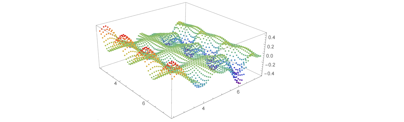
The overall cost optimization will look something like this:
$$ \text{Total cost} = \sum \text{distance all visited notes} + \text{penalties if not all constraints are met} $$
If we want to minimize the Total cost we have be use the most efficient route. This means getting a short route, but with all the constraints satisfied.
What we want to do with a QUBO, is formulating the optimization problem in a way that only uses variables that can take the value \(0\) or \(1\).
Let's dig in, a quick warning it will get a bit mathematical. A complete walkthrough with code is here. But let's explain each part of the total cost here bit by bit:
Total distance all visited notes
Let's start with a more generalized form of the distance matrix, our starting point:
$$ C = \begin{bmatrix} c_{1,1} & c_{1,2} & \dots & c_{1,N} \\ c_{2,1} & c_{2,2} & \dots & c_{2,N} \\ \vdots & \ddots & \ddots & \vdots \\ c_{N,1} & c_{N,2} & \dots & c_{N,N} \end{bmatrix} $$
To get the distance between two points we can actually use two vectors, like below. With this we can select the distance between any two points. This would mean that all values in the vectors are zero, except for the selected location that will be one. Using the matrix below if \(x_1\) and \(x_{N+1}\) will let you get the value of \(c_{1,2}\)
$$ \text{Cost for single trip }= \overbrace{\begin{bmatrix} x_1 & x_2 & \dots & x_N \end{bmatrix}}^{\text{origin selector} = X} \overbrace{ \begin{bmatrix} c_{1,1} & c_{1,2} & \dots & c_{1,N} \\ c_{2,1} & c_{2,2} & \dots & c_{2,N} \\ \vdots & \ddots & \ddots & \vdots \\ c_{N,1} & c_{N,2} & \dots & c_{N,N} \end{bmatrix}}^{\text{Cost matrix}=C} \overbrace{\begin{bmatrix} x_{N+1} \\ x_{N+2} \\ \vdots \\ x_{2N} \end{bmatrix}}^{\text{Destination selector} = Y} $$
Now, we want to get the total cost of driving to multiple places. Let's start by naming our origin matrix as \(X\) and the destination vector as \(Y\). To get the total cost of a route with \(N\) nodes we can formulate that as follows:
$$\text{Cost of route} = \sum_{k=1}^{N+1}\sum_{i=1}^{N}\sum_{j=1}^{N} \left( X_{N(k+1)+i}\cdot C_{i,j}\cdot Y_{Nk+j} \right)$$
To see how this can be coded with Azure Quantum Inspired Optimization take a look here.
With this we can calculate the total cost of a route, however when we do not apply constraints the solver might just stay in the same place to minimize cost. To make sure we visit all the nodes and have a valid route we need to add some constraints. Below we will explain all constraints which needed to create a valid route.
One location at a time constrain
In the previous section we described a method that can find the total cost for a set of locations. However this won't just give the right solution, since we want to penalize the solver if the solution is not valid. With we lower the probility that the solver will choose an invalid solution.
The first constrained that we want to add is that the salesperson can only be in a single position at any time.
How can we make sure that the salesperson is only in a single place at any moment in time? The answers lies within the origin and destination selector vectors. If we have a 3 node system and we are in place 1 the origin selector would look like this:
$$ \begin{bmatrix} x_1 & x_2 & x_3 \end{bmatrix} = \begin{bmatrix} 0 & 1 & 0 \end{bmatrix} $$
An invalid selection would be:
$$ \begin{bmatrix} x_1 & x_2 & x_3 \end{bmatrix} = \begin{bmatrix} 1 & 1 & 0 \end{bmatrix} \\ \text{or} \\ \begin{bmatrix} x_1 & x_2 & x_3 \end{bmatrix} = \begin{bmatrix} 0 & 0 & 0 \end{bmatrix} $$
To generalize we could say that we need to satisfy the following equations:
$$ x_1 \cdot x_2 = 0 \\ x_1 \cdot x_3 = 0 \\ x_2 \cdot x_3 = 0$$
These equations are only valid if there's only one single \(1\) value and the others are \(0\). If this is not the case we will give an extra penalty to the solver. This means that the solver will have lower probability to pick this solution.
Now we want to write this in a more generalized form and create the code to submit to the solver. The generalized form of this constrained will be:
$$ \sum_{l=1}^{N+1} \sum_{i=1}^{N} \sum_{j=1}^{N} X_{i+N(l-1)} \cdot X_{j+N(l-1)} $$
Here is the code for the solver and a more detailed description on this constraint.
At least one location at the time
In the previous constrained we tried to make sure that the salesperson was not in multiple locations at a single time. However, if you looked closely you might have noticed that the equations above would be satisfied if the sales person is not in a single location at all. Therefore we need to make a constrained that the salesperson is in at least one location at the time.
$$ 0 = (N+1) -\left( \sum_{k=1}^{N(N+1)} x_k \right) $$
This constraint will make sure that the salesperson is always at a location. This constraint can also be satisfied if the sales person would be in all locations at once, however the other constraints will make sure that this will not be a valid solution.
A more detailed description and code can be found here.
Visit all locations
Now we have three cost functions, one will calculate the complete distance of the route. The second will make sure the driver is only in a single place at each time and the last will make sure we are in at least one location. Next, we need to make sure that all locations are visited.
To add this constraint we take the similar approach as the previous constraints. Let's start with our location selector:
$$ \begin{bmatrix} x_1 & x_2 & x_3 \end{bmatrix} $$
We need to visit all these nodes once (let's discard for now that we need to travel back to the starting point). This means that if we have 3 time moments which we can call \(N\) and we want to make sure sure that we visit node \(x_1\) only once, the following needs to be satisfied:
$$ x_1 \cdot x_{1+N} =0 \\ x_1 \cdot x_{1+2N} = 0 $$
If at two different time moments \(N\) the location \(x_1\) has value \(1\), the equations above will not be satisfied, in this case we will give the solver a big penalty.
Start and stop at a specific node
Lastly, to complete the route we want to say where we want to start and stop our route. This is done by adding negative weights, a positive stimuli for the solver, for these locations. Here you can see how this is done in the code.
Now we have a complete system to calculate the perfect route. Note that when calculating the perfect route the solver might not always find the perfect solution. With tuning which is discussed later, you can try to improve the solutions.
Submit the Problem to Azure Quantum
With the cost functions defined, we can now send this to the Azure Quantum Inspired Optimization service. The service will take all the cost and the indices of each cost and solve for the most efficient route.
You will find that tweaking parameters, solver types and hardware can make a big difference on the performance of a solution. With the broad range of solvers and hardware there will be a great solver for each problem. Especially when problems grow using FPGA's will greatly reduce your solving time.
Tuning
When looking at the code, you see that some weights are multiplied by fixed numbers. These numbers can be used to tune the problem landscape. When you are building these optimization problems you will notice that these parameters can have a huge impact on the performance of the solution and/or solving time. So always play around with these when the solution is not as desired or slow. Also keep in mind that different solver types can have different sweet spots for these parameters.
Wrapping up
Here I have shown you how to tackle a common optimization problem using Azure Quantum Inspired Optimization. This type of optimization can be applied to lots of other problems like portfolio optimization, scheduling problems and more. All the code for this can be found here. If you have any comments please let me know below.